728x90
반응형
# 평가 지표
-회귀
- 평균 오차
-분류
- 정확도
- 오차행렬
- 정밀도
- 재현율
- F1스코어
- ROC AUC
3. 정밀도와 재현율 (Precision과 Recall)
- 불균형한 데이터 세트에서 정확도보다 더 선호되는 평가 지표
- positive 데이터 세트의 예측 성능에 초점을 맞춘 평가 지표
- 재현율과 정밀도 모두 TP를 높이는 데 동일한 초점임 BUT 재현율은 FN을 낮추고, 정밀도는 FP를 낮추는데 초점
- 가장 좋은 성능 평가는 재현율, 정밀도 모두 높은 수치를 얻는 것. 반면 둘 중 하나만 높고 하나만 낮은 결과일 경우 바람직하지 않음)
정밀도 = TP / (FP +TP )
- 정밀도가 더 중요한 경우 : 실제 Negative 음성인 데이터 예측을 Positive 양성으로 잘못 판단하게 될 경우
- ( ex. 스팸메일이 아닌데(negative) 스팸메일 (Positive )이라고 분류하는 경우 )
재현율 = TP / ( FN +TP )
- 재현율이 더 중요한 경우 : 실제 Positive인 데이터 예측을 Negative 음성으로 잘못 판단하게 될 경우
- ( ex. 암인 사람(Positive) 을 암이 아니라고(negative) 분류 하는 경우)
from sklearn.metrics import accuracy_score, precision_score , recall_score , confusion_matrix

def get_clf_eval(y_test , pred):
    confusion = confusion_matrix( y_test, pred) # 오차행렬
    accuracy = accuracy_score(y_test , pred) # 정확도
    precision = precision_score(y_test , pred) # 정밀도
    recall = recall_score(y_test , pred) # 재현율
    print('오차 행렬')
    print(confusion)
    print('정확도: {0:.4f}, 정밀도: {1:.4f}, 재현율: {2:.4f}'.format(accuracy , precision ,recall))
import numpy as np
import pandas as pd
from sklearn.model_selection import train_test_split
from sklearn.linear_model import LogisticRegression
# 원본 데이터를 재로딩, 데이터 가공, 학습데이터/테스트 데이터 분할.
titanic_df = pd.read_csv('./titanic_train.csv')
y_titanic_df = titanic_df['Survived']
X_titanic_df= titanic_df.drop('Survived', axis=1)
X_titanic_df = transform_features(X_titanic_df)
X_train, X_test, y_train, y_test = train_test_split(X_titanic_df, y_titanic_df, \
test_size=0.20, random_state=11)
lr_clf = LogisticRegression()
lr_clf.fit(X_train , y_train)
pred = lr_clf.predict(X_test)
get_clf_eval(y_test , pred)오차 행렬
[[104 14]
[ 13 48]]
정확도: 0.8492, 정밀도: 0.7742, 재현율: 0.7869
# 정밀도/재현율 트레이드 오프 (임계값 사용 X)
정밀도와 재현율은 상호 보완적인 평가지표이기 때문에 하나가 오르면 다른 하나의 수치는 떨어지기 쉽다. 이를 정밀도/재현율의 트레이드오프라고 부른다.
pred_proba = lr_clf.predict_proba(X_test)
pred = lr_clf.predict(X_test)
print('pred_proba()결과 Shape : {0}'.format(pred_proba.shape))
print('pred_proba array에서 앞 3개만 샘플로 추출 \n:', pred_proba[:3])
# 예측 확률 array 와 예측 결과값 array 를 concatenate 하여 예측 확률과 결과값을 한눈에 확인
pred_proba_result = np.concatenate([pred_proba , pred.reshape(-1,1)],axis=1)
print('두개의 class 중에서 더 큰 확률을 클래스 값으로 예측 \n',pred_proba_result[:3])pred_proba()결과 Shape : (179, 2)
pred_proba array에서 앞 3개만 샘플로 추출
: [[0.46162417 0.53837583] # => 클래스 0일 확률 , 클래스 1일 확률
[0.87858538 0.12141462]
[0.87723741 0.12276259]]
두개의 class 중에서 더 큰 확률을 클래스 값으로 예측
[[0.46162417 0.53837583 1. ] # 0.4<0.5 이므로 1
[0.87858538 0.12141462 0. ] # => 0.8>0.1 이므로 클래스 0
[0.87723741 0.12276259 0. ]]
+ 확인용 코드
print(pred_proba[:3])
print(pred[:3])[[0.46162417 0.53837583]
[0.87858538 0.12141462]
[0.87723741 0.12276259]]
[1 0 0]
# 정밀도/재현율 트레이드 오프 (임계값 사용 O)
from sklearn.preprocessing import Binarizer
custom_threshold = 0.5 # 임계값 설정
# predict_proba( ) 반환값의 두번째 컬럼 추출 후 행렬로 변환,
# 즉 Positive 클래스 컬럼 하나만 추출하여 Binarizer를 적용
pred_proba_1 = pred_proba[:,1].reshape(-1,1)
binarizer = Binarizer(threshold=custom_threshold).fit(pred_proba_1)
custom_predict = binarizer.transform(pred_proba_1)
get_clf_eval(y_test, custom_predict)오차 행렬
[[104 14]
[ 13 48]]
정확도: 0.8492, 정밀도: 0.7742, 재현율: 0.7869=> 임계값 0.5 일때의 결과
# 임계값을 0.5에서 0.4로 낮춤
custom_threshold = 0.4
pred_proba_1 = pred_proba[:,1].reshape(-1,1)
binarizer = Binarizer(threshold=custom_threshold).fit(pred_proba_1)
custom_predict = binarizer.transform(pred_proba_1)
get_clf_eval(y_test , custom_predict)오차 행렬
[[99 19]
[10 51]]
정확도: 0.8380, 정밀도: 0.7286, 재현율: 0.8361=> 임계값 0.4로 낮추었을때의 결과
# 임계값을 낮추니 재현율이 올라가고 정밀도가 떨어졌음
: 임계값은 Positive예측값을 결정하는 확률의 기준이 됨. 그렇기 때문에 0.5가 아닌 0.4부터 positive로 예측을 너그럽게 하기 때문에 임계값 값을 낮출수록 True값이 많아지게 되는 것
# 테스트를 수행할 모든 임곗값을 리스트 객체로 저장.
thresholds = [0.4, 0.45, 0.50, 0.55, 0.60]
def get_eval_by_threshold(y_test , pred_proba_c1, thresholds):
# thresholds list객체내의 값을 차례로 iteration하면서 Evaluation 수행.
for custom_threshold in thresholds:
binarizer = Binarizer(threshold=custom_threshold).fit(pred_proba_c1)
custom_predict = binarizer.transform(pred_proba_c1)
print('임곗값:',custom_threshold)
get_clf_eval(y_test , custom_predict)
get_eval_by_threshold(y_test ,pred_proba[:,1].reshape(-1,1), thresholds )임곗값: 0.4
오차 행렬
[[99 19]
[10 51]]
정확도: 0.8380, 정밀도: 0.7286, 재현율: 0.8361
임곗값: 0.45
오차 행렬
[[103 15]
[ 12 49]]
정확도: 0.8492, 정밀도: 0.7656, 재현율: 0.8033
임곗값: 0.5
오차 행렬
[[104  14]
 [ 13  48]]
정확도: 0.8492, 정밀도: 0.7742, 재현율: 0.7869
임곗값: 0.55
오차 행렬
[[109 9]
[ 15 46]]
정확도: 0.8659, 정밀도: 0.8364, 재현율: 0.7541
임곗값: 0.6
오차 행렬
[[112 6]
[ 16 45]]
정확도: 0.8771, 정밀도: 0.8824, 재현율: 0.7377
임계값을 사용하는 사이킷런 API : precision_recall_curve()
from sklearn.metrics import precision_recall_curve

# 레이블 값이 1일때의 예측 확률을 추출
pred_proba_class1 = lr_clf.predict_proba(X_test)[:, 1]

# 실제값 데이터 셋과 레이블 값이 1일 때의 예측 확률을 precision_recall_curve 인자로 입력
precisions, recalls, thresholds = precision_recall_curve(y_test, pred_proba_class1 )
print('반환된 분류 결정 임곗값 배열의 Shape:', thresholds.shape)

#반환된 임계값 배열 로우가 147건이므로 샘플로 10건만 추출하되, 임곗값을 15 Step으로 추출.
thr_index = np.arange(0, thresholds.shape[0], 15)
print('샘플 추출을 위한 임계값 배열의 index 10개:', thr_index)
print('샘플용 10개의 임곗값: ', np.round(thresholds[thr_index], 2))

# 15 step 단위로 추출된 임계값에 따른 정밀도와 재현율 값
print('샘플 임계값별 정밀도: ', np.round(precisions[thr_index], 3))
print('샘플 임계값별 재현율: ', np.round(recalls[thr_index], 3))
반환된 분류 결정 임곗값 배열의 Shape: (143,)
샘플 추출을 위한 임계값 배열의 index 10개: [ 0 15 30 45 60 75 90 105 120 135]
샘플용 10개의 임곗값: [0.1 0.12 0.14 0.19 0.28 0.4 0.56 0.67 0.82 0.95]
샘플 임계값별 정밀도: [0.389 0.44 0.466 0.539 0.647 0.729 0.836 0.949 0.958 1. ]
샘플 임계값별 재현율: [1. 0.967 0.902 0.902 0.902 0.836 0.754 0.607 0.377 0.148]
# 임계값 변화에 따른 정밀도와 재현율 그래프
import matplotlib.pyplot as plt
import matplotlib.ticker as ticker
%matplotlib inline

def precision_recall_curve_plot(y_test , pred_proba_c1):
    # threshold ndarray와 이 threshold에 따른 정밀도, 재현율 ndarray 추출.
    precisions, recalls, thresholds = precision_recall_curve( y_test, pred_proba_c1)

    # X축을 threshold값으로, Y축은 정밀도, 재현율 값으로 각각 Plot 수행. 정밀도는 점선으로 표시
    plt.figure(figsize=(8,6))
    threshold_boundary = thresholds.shape[0]
    plt.plot(thresholds, precisions[0:threshold_boundary], linestyle='--', label='precision')
    plt.plot(thresholds, recalls[0:threshold_boundary],label='recall')

    # threshold 값 X 축의 Scale을 0.1 단위로 변경
    start, end = plt.xlim()
    plt.xticks(np.round(np.arange(start, end, 0.1),2))

    # x축, y축 label과 legend, 그리고 grid 설정
    plt.xlabel('Threshold value'); plt.ylabel('Precision and Recall value')
    plt.legend(); plt.grid()
    plt.show()

precision_recall_curve_plot( y_test, lr_clf.predict_proba(X_test)[:, 1] )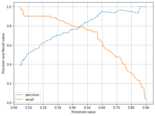
728x90
반응형
'pythonML' 카테고리의 다른 글
| [pythonML] 부스팅(Boosting)-LGBM(Light Gradient Boost Machine) (0) | 2022.07.15 |
|---|---|
| [pythonML] ROC곡선과 AUC , F1스코어 - 평가 (0) | 2022.07.11 |
| [pythonML] 정확도와 오차행렬 - 평가 (0) | 2022.07.10 |
| [pythonML] 회귀- LinearRegression (0) | 2022.05.09 |
| [pythonML] 회귀- 경사하강법 (0) | 2022.04.17 |